
Some images do not typically carry coordinate information; therefore, units, scales and pixel sizes of projects can be set manually in two ways:
The default unit of a project with no resolution information is a pixel. For these projects, the pixel size cannot be altered. Once a unit is defined in a project, any number or features within a rule set can be used with a defined unit. Here the following rules apply:
Since ‘same as project unit’ might vary with the project, we recommend using absolute units.
Thematic layers are raster or vector files that have associated attribute tables, which can add additional information to an image. For instance, a satellite image could be combined with a thematic layer that contains information on the addresses of buildings and street names. They are usually used to store and transfer results of an image analysis.
Thematic vector layers comprise only polygons, lines or points. While image layers contain continuous information, the information of thematic raster layers is discrete. Image layers and thematic layers must be treated differently in both segmentation and classification.
Typically – unless you have created them yourself – you will have acquired a thematic layer from an external source. It is then necessary to import this file into your project. eCognition Developer supports a range of thematic formats and a thematic layer can be added to a new project or used to modify an existing project.
Thematic layers can be specified when you create a new project via File > New Project – simply press the Insert button by the Thematic Layer pane. Alternatively, to import a layer into an existing project, use the File > Modify Existing Project function or select File > Add data Layer. Once defined, the Edit button allows you to further modify the thematic layer and the Delete button removes it.
When importing thematic layers, ensure the image layers and the thematic layers have the same coordinate systems and geocoding. If they do not, the content of the individual layers will not match.
As well as manually importing thematic layers, using the File > New Project or File > Modify Open Project dialog boxes, you can also import them using rule sets. For more details, look up the Create/Modify Project algorithm in the eCognition Developer Reference Book.
The polygon shapefile (.shp), which is a common format for geo-information systems, will import with its corresponding thematic attribute table file (.dbf) file automatically. For all other formats, the respective attribute table must be specifically indicated in the Load Attribute Table dialog box, which opens automatically. From the Load Attribute Table dialog box, choose one of the following supported formats:
When loading a thematic layer from a multi-layer image file (for example an .img stack file), the appropriate layer that corresponds with the thematic information is requested in the Import From Multi Layer Image dialog box. Additionally, the attribute table with the appropriate thematic information must be loaded.
If you import a thematic layer into your project and eCognition Developer does not find an appropriate column with the caption ID in the respective attribute table, the Select ID Column dialog box will open automatically. Select the caption of the column containing the polygon ID from the drop-down menu and confirm with OK.
All thematic layers can be activated and inactivated for display via the Vector Layers checkbox, or individually using the respective checkbox of a single vector layer.
The values of thematic objects are displayed in the Thematic Layer Attribute Table, which is launched via Tools > Thematic Layer Attribute Table.
To view the thematic attributes, open the Manual Editing toolbar. Choose Thematic Editing as the active editing mode and select a thematic layer from the Select Thematic Layer drop-down list.
The attributes of the selected thematic layer are now displayed in the Thematic Layer Attribute Table. They can be used as features in the same way as any other feature provided by eCognition.
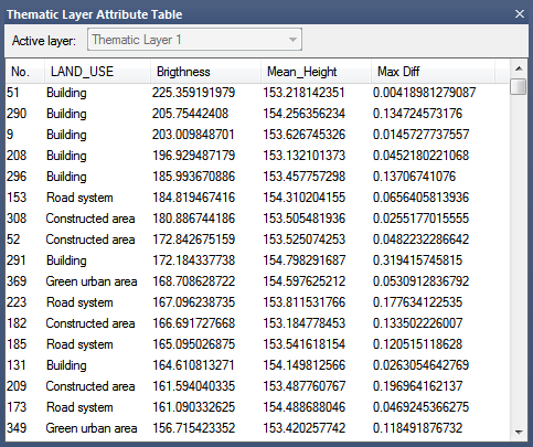
The table supports integers, strings, and doubles. The column type is set automatically, according to the attribute, and table column widths can be up to 255 characters.
Class name and class color are available as features and can be added to the Thematic Layer Attribute Table window. You can modify the thematic layer attribute table by adding, editing or deleting table columns or editing table rows.
A thematic object is the basic element of a thematic layer and can be a polygon, line or point. It represents positional data of a single object in the form of coordinates and describes the object by its attributes.
The Manual Editing toolbar lets you manage thematic objects, including defining regions of interest before image analysis and the verification of classifications after image analysis.
If you want to edit image objects instead of thematic objects by hand, choose Image Object Editing from the drop-down list.
While editing image objects manually is not commonly used in automated image analysis, it can be applied to highlight or reclassify certain objects, or to quickly improve the analysis result without adjusting a rule set. The primary manual editing tools are for merging, classifying and cutting manually.
To display the Manual Editing toolbar go to View > Toolbars > Manual Editing from the main menu. Ensure the editing mode, displayed in the Change Editing Mode drop-down list, is set to Image Object Editing.
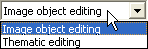
If you want to edit thematic objects by hand, choose Thematic Editing from the drop-down list.
If you do not use an existing layer to work with thematic objects, you can create a new one. For example, you may want to define regions of interest as thematic objects and export them for later use with the same or another project.
On the Select Thematic Layer drop-down menu, select New Layer to open the Create New Thematic Layer dialog box. Enter an name and select the type of thematic vector layer: polygon, line or point layer.
There are two ways to generate new thematic objects – either use existing image objects or create them yourself. This may either be based on an existing layer or on a new thematic layer you have created.
For all objects, the selected thematic layer must be set to the appropriate selection: polygon, line or point. Pressing the Generate Thematic Objects button on the Manual Editing toolbar will then open the appropriate window for shape creation. The Single Selection button is used to finish the creation of objects and allows you to edit or delete them.
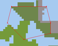
To draw polygons go to the Change Editing Mode drop-down menu and change the editing mode to Thematic Editing. Now in the Select thematic layer drop-down select - New Layer -. In the upcoming dialog choose Type: Polygon Layer. Activate the Generate Thematic Objects button and click in the view to set vertices. Double click to complete the shape or right-click and select Close Polygon from the context menu. This object can touch or cross any existing image object.
The following cursor actions are available:
To draw lines go to the Change Editing Mode drop-down menu and change the editing mode to Thematic Editing. Now in the Select thematic layer drop-down select - New Layer -. In the upcoming dialog choose Type: Line Layer. Activate the Generate Thematic Objects button and click in the view to set vertices in the thematic line layer. Double click to complete the line or right-click and choose End Line to stop drawing. This object can touch or cross any existing image object.
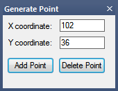
To generate points select thematic layer type: Point Layer and add points in one of the following ways:
The point objects can touch any existing image object. To delete the point whose coordinates are displayed in the Generate Point dialog box, press Delete Point.
Note that image objects can be converted to thematic objects automatically using the algorithm convert image objects to vector objects.
Thematic objects can be created manually from the outlines of selected image objects. This function can be used to improve a thematic layer – new thematic objects are added to the Thematic Layer Attribute Table. Their attributes are initially set to zero.
Use the Classify Selection context menu command if you want to classify image objects manually. Note, that you have to Select a Class for Manual Classification with activated Image object editing mode beforehand.

Image objects or thematic objects can be selected using these buttons on the Manual Editing toolbar. From left to right:
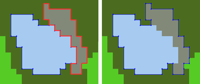
You can merge objects manually, although this function only operates on the current image object level. To merge neighboring objects into a new single object, choose Tools > Manual Editing > Merge Objects from the main menu or press the Merge Objects Manually button on the Manual Editing toolbar to activate the input mode.
Select the neighboring objects to be merged in map view. Selected objects are displayed with a red outline (the color can be changed in View > Display Mode > Edit Highlight Colors).
To clear a selection, click the Clear Selection for Manual Object Merging button or deselect individual objects with a single mouse-click. To combine objects, use the Merge Selected Objects button on the Manual Editing toolbar, or right-click and choose Merge Selection.
If an object cannot be activated, it cannot be merged with the already selected one because they do not share a common border. In addition, due to the hierarchical organization of the image objects, an object cannot have two superobjects. This limits the possibilities for manual object merging, because two neighboring objects cannot be merged if they belong to two different superobjects.
You can create merge the outlines of a thematic object and an image object while leaving the image object unchanged:
To cut a single image object or thematic object:
If you cut image objects, note that the Cut Objects Manually tool cuts both the selected image object and its sub-objects on lower image object levels.

Thematic objects, with their accompanying thematic layers, can be exported to vector shapefiles. This enables them to be used with other maps or projects.
In the manual editing toolbar, select Save Thematic Layer As, which exports the layer in .shp format. Alternatively, you can use the Export Results dialog box.
In contrast to image layers, thematic layers contain discrete information. This means that related layer values can carry additional information, defined in an attribute list.
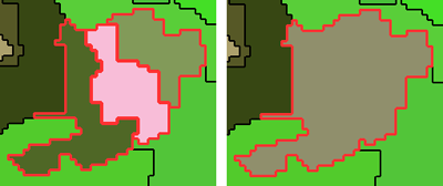
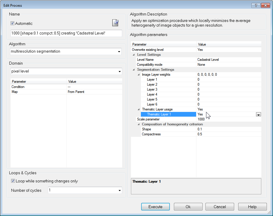
The affiliation of an object to a class in a thematic layer is clearly defined, it is not possible to create image objects that belong to different thematic classes. To ensure this, the borders separating different thematic classes restrict further segmentation whenever a thematic layer is used during segmentation. For this reason, thematic layers cannot be given different weights, but can merely be selected for use or not.
If you want to produce image objects based exclusively on thematic layer information, you have to switch the weights of all image layers to zero. You can also segment an image using more than one thematic layer. The results are image objects representing proper intersections between the layers.
Within rule sets you can use variables in different ways. Some common uses of variables are:
While developing rule sets, you commonly use scene and object variables for storing your dedicated fine-tuning tools for reuse within similar projects.
Variables for classes, image object levels, features, image layers, thematic layers, maps and regions enable you to write rule sets in a more abstract form. You can create rule sets that are independent of specific class names or image object level names, feature types, and so on.
Scene variables are global variables that exist only once within a project. They are independent of the current image object.
Object variables are local variables that may exist separately for each image object. You can use object variables to attach specific values to image objects.
Class Variables use classes as values. In a rule set they can be used instead of ordinary classes to which they point.
Feature Variables have features as their values and return the same values as the feature to which they point.
Level Variables have image object levels as their values. Level variables can be used in processes as pointers to image object levels.
Image Layer and Thematic Layer Variables have layers as their values. They can be selected whenever layers can be selected, for example, in features, domains, and algorithms. They can be passed as parameters in customized algorithms.
Region Variables have regions as their values. They can be selected whenever layers can be selected, for example in features, domains and algorithms. They can be passed as parameters in customized algorithms.
Map Variables have maps as their values. They can be selected wherever a map is selected, for example, in features, domains, and algorithm parameters. They can be passed as parameters in customized algorithms.
Feature List lets you select which features are exported as statistics.
The Image Object List lets you organize image objects into lists and apply functions to these lists.
To open the Manage Variables box, go to the main menu and select Process > Manage Variables, or click the Manage Variables icon on the Tools toolbar.
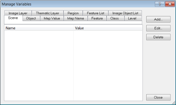
Select the tab for the type of variable you want to create then click Add. A Create Variable dialog box opens, with particular fields depending on which variable is selected.
Selecting scene or object variables launches the same Create Variable dialog box.
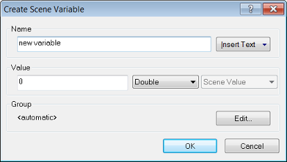
The Name and Value fields allow you to create a name and an initial value for the variable. In addition you can choose whether the new variable is numeric (double) or textual (string).
The Insert Text drop-down box lets you add patterns for rule set objects, allowing you to assign more meaningful names to variables, which reflect the names of the classes and layers involved. The following feature values are available: class name; image layer name; thematic layer name; variable value; variable name; level name; feature value.
The Type field is unavailable for both variables. The Shared check-box allows you to share the new variable among different rule sets.
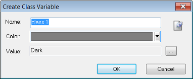
The Name field and comments button are both editable and you can also manually assign a color.
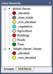
To give the new variable a value, click the ellipsis button to select one of the existing classes as the value for the class variable. Click OK to save the changes and return to the Manage Variables dialog box. The new class variable will now be visible in the Feature Tree and the Class Hierarchy, as well as the Manage Variables box.
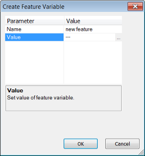
After assigning a name to your variable, click the ellipsis button in the Value field to open the Select Single Feature dialog box and select a feature as a value.
After you confirm the variable with OK, the new variable displays in the Manage Variables dialog box and under Feature Variables in the feature tree in several locations, for example, the Feature View window and the Select Displayed Features dialog box
Region Variables have regions as their values and can be created in the Create Region Variable dialog box. You can enter up to three spatial dimensions and a time dimension. The left hand column lets you specify a region’s origin in space and the right hand column its size.
The new variable displays in the Manage Variables dialog box, and wherever it can be used, for example, as a domain parameter in the Edit Process dialog box.
Create Level Variable allows the creation of variables for image object levels, image layers, thematic layers, maps or regions.
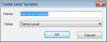
The Value drop-down box allows you to select an existing level or leave the level variable unassigned. If it is unassigned, you can use the drop-down arrow in the Value field of the Manage Variables dialog box to create one or more new names.
Parameter sets are storage containers for specific variable value settings. They are mainly used when creating action libraries, where they act as a transfer device between the values set by the action library user and the rule set behind the action. Parameter sets can be created, edited, saved and loaded. When they are saved, they store the values of their variables; these values are then available when the parameter set is loaded again.
To create a parameter set, go to Process > Manage Parameter Sets
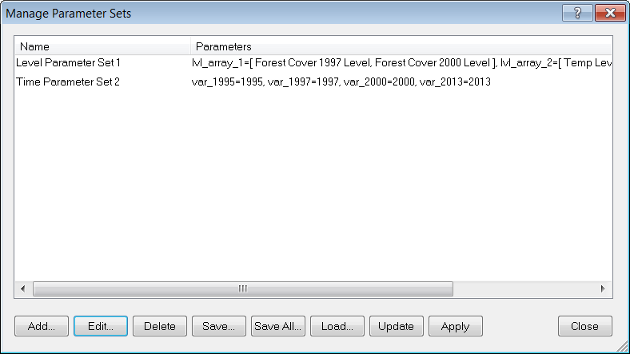
In the dialog box click Add. The Select Variable for Parameter Set dialog box opens. After adding the variables the Edit Parameter Set dialog box opens with the selected variables displayed.
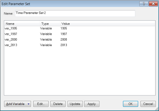
Insert a name for your new parameter set and confirm with OK.
You can edit a parameter set by selecting Edit in the Manage Parameter Sets dialog box:
Actions #4 and #5 may change your rule set.
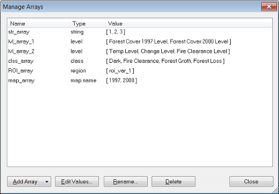
The array functions in eCognition Developer let you create lists of features, which are accessible from all rule set levels. This allows rule sets to be repeatedly executed across, for example, classes, levels and maps.
The Manage Arrays dialog box can be accessed via Process > Manage Arrays in the main menu. The following types of arrays are supported: numbers; strings; classes; image layers; thematic layers; levels; features; regions; map names.
To add an array, press the Add Array button and select the array type from the drop-down list. Where arrays require numerical values, multiple values must be entered individually by row. Using this dialog, array values – made up of numbers and strings – can be repeated several times; other values can only be used once in an array. Additional values can be added using the algorithm Update Array, which allows duplication of all array types.
When selecting arrays such as level and image layer, hold down the Ctrl or Shift key to enter more than one value. Values can be edited either by double-clicking them or by using the Edit Values button.
Initially, string, double, map and region arrays are executed in the order they are entered. However, the action of rule sets may cause this order to change.
Class and feature arrays are run in the order of the elements in the Class Hierarchy and Feature Tree. Again, this order may be changed by the actions of rule sets; for example a class or feature array may be sorted by the algorithm Update Array, then the array edited in the Manage Array dialog at a later stage – this will cause the order to be reset and duplicates to be removed.
‘Array’ can be selected in all Process-Related Operations (other than Execute Child Series).
In any algorithm where it is possible to enter a value or variable parameter, it is possible to select an array item.
In Scene Features > Rule set-related, three array variables are present: rule set array values, rule set array size and rule set array item. For more information, please consult the Reference Book.
Rule set arrays may be used as parameters in customized algorithms.
Arrays may be selected in the Find What box in the Find and Replace pane.
Through the examples in earlier chapters, you will already have some familiarity with the idea of parent and child domains, which were used to organize processes in the Process Tree. In that example, a parent object was created which utilized the Execute Child Processes algorithm on the child processes beneath it.
Below is a list of terms used in the context of process hierarchy
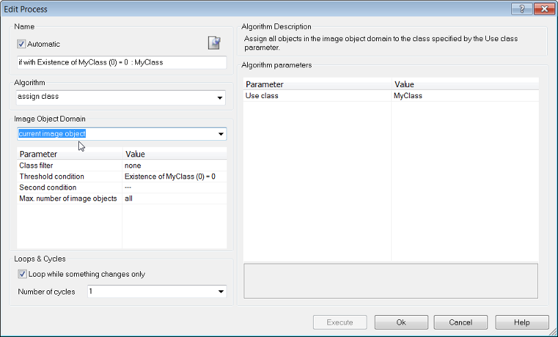
A parent process object (PPO) is an image object to which a child process refers and must first be defined in the parent process. An image object can be called through the respective selection in the Edit Process dialog box; go to the Domain group box and select one of the four local processing options from the drop-down list, such as current image object.
When you use local processing, the routine goes to the first random image object described in the parent domain and processes all child processes defined under the parent process, where the PPO is always that same image object.
The routine then moves through every image object in the parent domain. The routine does not update the parent domain after each processing step; it will continue to process those image objects found to fit the parent process’s domain criteria, no matter if they still fit them when they are to be executed.
A special case of a PPO is the 0th order PPO, also referred to as PPO(0). Here the PPO is the image object defined in the domain in the same line (0 lines above).
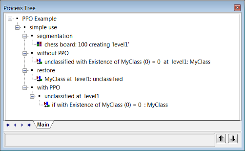
For better understanding of child domains (subdomains) and PPOs, see the example below.
This example demonstrates how local processing is used to change the order in which class or feature filters are applied. During execution of each process line, eCognition software first creates internally a list of image objects that are defined in the domain. Then the desired routine is executed for all image objects on the list.
ParentProcessObjects.dpr
no My Class objects exist in the neighborhood are split into two different lines. at Level 1: Unclassified (restore) removes the classification and returns to the state after step 3. The process if with Existence of My Class (0) = 0:My Class applies the algorithm Assign Class to the image object that has been set in the parent process unclassified at Level 1: for all. This has been invoked by selecting Current Image Object as domain. Therefore, all unclassified image objects will be called sequentially and each unclassified image object will be treated separately.
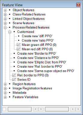
One more powerful tool comes with local processing. When a child process is executed, the image objects in the domain ‘know’ their parent process object (PPO). It can be very useful to directly compare properties of those image objects with the properties of the PPO. A special group of features, the process-related features, do exactly this job.
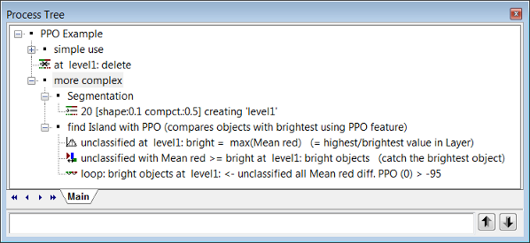
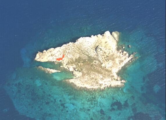
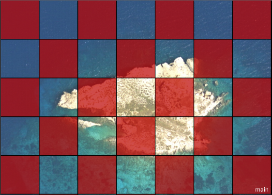
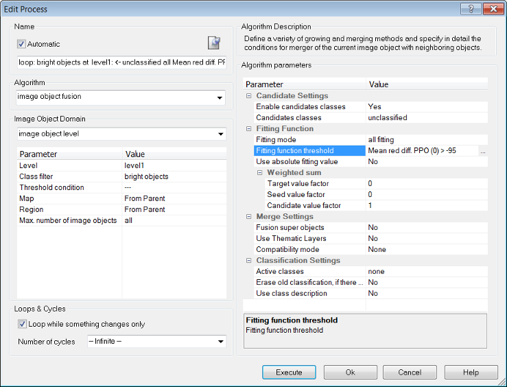
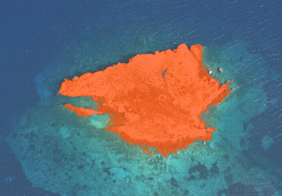
more complex is executed. After the Segmentation the visualization settings are switched to the outline view. In this rule set the PPO(0) procedure is used to merge the image objects with the brightest image object classified as bright objects in the red image layer. For this purpose a difference range (> −95) to an image object of the class bright objects is used. bright objects) is the brightest image object in this image. To find out how it is different from similar image objects to be merged with, the user has to select it using the Ctrl key. Doing that the parent process object (PPO) is manually selected. The PPO will be highlighted in green.bright objects) the values in the Image Object Information window can be checked. The green highlighted image object displays the PPO. All other image objects that are selected will be highlighted in red and you can view the difference from the green highlighted image object in the Image Object Information window . Now you can see the result of the image object fusion.

Customized features can be arithmetic or relational (relational features depend on other features). All customized features are based on the features of eCognition Developer.
The Manage Customized Features dialog box allows you to add, edit, copy and delete customized features, and to create new arithmetic and relational features based on the existing ones.
To open the dialog box, click on Tools > Manage Customized Features from the main menu, or click the icon on the Tools toolbar.
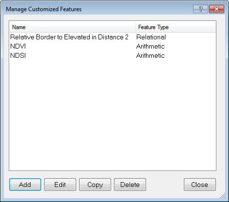
Clicking the Add button launches the Customized Features dialog box, which allows you to create a new feature. The remaining buttons let you to edit, copy and delete features.
The procedure below guides you through the steps you need to follow when you want to create an arithmetic customized feature.
Open the Manage Customized Features dialog box and click Add. Select the Arithmetic tab in the Customized Features dialog box.

The calculator buttons are arranged in a standard layout. In addition:
 ) or a square root (x^0.5 for
  ).
).  .
.The following procedure will assist you with the creation of a relational customized feature.

Relations between surrounding objects can exist either on the same level or on a level lower or higher in the image object hierarchy:
| Object | Description |
|---|---|
| Neighbors | Related image objects on the same level. If the distance of the image objects is set to 0 then only the direct neighbors are considered. When the distance is greater than 0 then the relation of the objects is computed using their centers of gravity. Only those neighbors whose center of gravity is closer than the distance specified from the starting image object are considered. The distance is calculated either in definable units or pixels. |
| Sub-objects | Image objects that exist below other image objects whose position in the hierarchy is higher (super-objects). The distance is calculated in levels. |
| Super-object | Contains other image objects (sub-objects) on lower levels in the hierarchy. The distance is calculated in levels. |
| Sub-objects of super-object | Only the image objects that exist below a specific superobject are considered in this case. The distance is calculated in levels. |
| Level | Specifies the level on which an image object will be compared to all other image objects existing at this level. The distance is calculated in levels. |
Overview of all functions existing in the drop-down list under the relational function section:
| Function | Description |
|---|---|
| Mean | Calculates the mean value of selected features of an image object and its neighbors. You can select a class to apply this feature or no class if you want to apply it to all image objects. Note that for averaging, the feature values are weighted with the area of the image objects. |
| Standard deviation | Calculates the standard deviation of selected features of an image object and its neighbors. You can select a class to apply this feature or no class if you want to apply it to all image objects. |
| Mean difference | Calculates the mean difference between the feature value of an image object and its neighbors of a selected class. Note that the feature values are weighted by either by the border length (distance =0) or by the area (distance >0) of the respective image objects. |
| Mean absolute difference | Calculates the mean absolute difference between the feature value of an image object and its neighbors of a selected class. Note that the feature values are weighted by either by the border length (distance =0) or by the area (distance >0)of the respective image objects. |
| Ratio | Calculates the proportion between the feature value of an image object and the mean feature value of its neighbors of a selected class. Note that for averaging the feature values are weighted with the area of the corresponding image objects. |
| Sum | Calculates the sum of the feature values of the neighbors of a selected class. |
| Number | Calculates the number of neighbors of a selected class. You must select a feature in order for this feature to apply, but it does not matter which feature you pick. |
| Min | Returns the minimum value of the feature values of an image object and its neighbors of a selected class. |
| Max | Returns the maximum value of the feature values of an image object and its neighbors of a selected class. |
| Mean difference to higher values | Calculates the mean difference between the feature value of an image object and the feature values of its neighbors of a selected class, which have higher values than the image object itself. Note that the feature values are weighted by either by the border length (distance =0) or by the area (distance > 0)of the respective image objects. |
| Mean difference to lower values | Calculates the mean difference between the feature value of an image object and the feature values of its neighbors of a selected class, which have lower values than the object itself. Note that the feature values are weighted by either by the border length (distance = 0) or by the area (distance >0) of the respective image objects. |
| Portion of higher value area | Calculates the portion of the area of the neighbors of a selected class, which have higher values for the specified feature than the object itself to the area of all neighbors of the selected class. |
| Portion of lower value area | Calculates the portion of the area of the neighbors of a selected class, which have lower values for the specified feature than the object itself to the area of all neighbors of the selected class. |
| Portion of higher values | Calculates the feature value difference between an image object and its neighbors of a selected class with higher feature values than the object itself divided by the difference of the image object and all its neighbors of the selected class. Note that the features are weighted with the area of the corresponding image objects. |
| Portion of lower values | Calculates the feature value difference between an image object and its neighbors of a selected class with lower feature values than the object itself divided by the difference of the image object and all its neighbors of the selected class. Note that the features are weighted with the area of the corresponding image object. |
| Mean absolute difference to neighbors | Available only if sub-objects is selected for Relational function concerning. Calculates the mean absolute difference between the feature value of sub-objects of an object and the feature values of a selected class. Note that the feature values are weighted by either by the border length (distance = 0) or by the area (distance > 0) of the respective image objects. |
You can save customized features separately for use in other rule sets:2
You can find customized features at different places in the feature tree, depending on the features to which they refer. For example, a customized feature that depends on an object feature is sorted below the group Object Features > Customized.
If a customized feature refers to different feature types, they are sorted in the feature tree according to the interdependencies of the features used. For example, a customized feature with an object feature and a class-related feature displays below class-related features.
You may wish to create a customized feature and display it in another part of the Feature Tree. To do this, go to Manage Customized Features and press Edit in the Feature Group pane. You can then select another group in which to display your customized feature. In addition, you can create your own group in the Feature Tree by selecting Create New Group. This may be useful when creating solutions for another user.
Although it is possible to use variables as part or all of a customized feature name, we would not recommend this practice as – in contrast to features – variables are not automatically updated and the results could be confusing.
Defining customized algorithms is a method of reusing a process sequence in different rule sets and analysis contexts. By using customized algorithms, you can split complicated procedures into a set of simpler procedures to maintain rule sets over a longer period of time.
You can specify any rule set item (such as a class, feature or variable) of the selected process sequence to be used as a parameter within the customized algorithm. A creation of configurable and reuseable code components is thus possible. A rule set item is any object in a rule set. Therefore, a rule set item can be a class, feature, image layer alias, level name or any type of variable.
Customized algorithms can be modified, which ensures that code changes take effect immediately in all relevant places in your rule set. When you want to modify a duplicated process sequence, you need to perform the changes consistently to each instance of this process. Using customized algorithms, you only need to modify the customized algorithm and the changes will affect every instance of this algorithm.
A rule set item is any object in a rule set other than a number of a string. Therefore, a rule set item can be a class, feature, image layer alias, level name or any type of variable. To restrict the visibility and availability of rule set items to a customized algorithm, local variables or objects can be created within a customized algorithm. Alternatively, global variables and objects are available throughout the complete rule set.
A rule set item in a customized algorithm can belong to one of the following scope types:
Rule set items can be grouped as follows, in terms of dependencies:
A relationship exists between dependencies of rule set items used in customized algorithms and their scope. If, for example, a process uses class A with a customized feature Arithmetic1, which is defined as local within the customized algorithm, then class A should also be defined as local. Defining class A as global or parameter can result in an inconsistent situation (for example a global class using a local feature of the customized algorithm).
Scope dependencies of rule set items used in customized algorithms are handled automatically according to the following consistency rules:
During the execution of a customized algorithm, image objects can refer to local rule set items. This might be the case if, for example, they get classified using a local class, or if a local temporary image object level is created. After execution, the references have to be removed to preserve the consistency of the image object hierarchy. The application offers two options to handle this cleanup process.
When Delete Local Results is enabled, the software automatically deletes locally created image object levels, removes all classifications using local classes and removes all local image object variables. However, this process takes some time since all image objects need to be scanned and potentially modified. For customized algorithms that are called frequently or that do not create any references, this additional checking may cause a significant runtime overhead. If not necessary, we therefore do not recommend enabling this option.
When Delete Local Results is disabled, the application leaves local image object levels, classifications using local classes and local image object variables unchanged. Since these references are only accessible within the customized algorithm, the state of the image object hierarchy might then no longer be valid. When developing a customized algorithm you should therefore always add clean-up code at the end of the procedure, to ensure no local references are left after execution. Using this approach, you will create customized algorithms with a much better performance compared to algorithms that relying on the automatic clean-up capability.
When a customized algorithm is called, the selected domain needs to be handled correctly. There are two options:
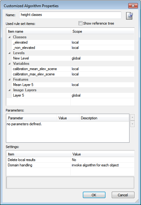

The local features and feature parameters are displayed in the feature tree of the Feature View window using the name of the customized algorithm, for example MyCustomizedAlgorithm.ArithmeticFeature1.
The local variables and variable parameters can be checked in the Manage Variables dialog box. They use the name of the customized algorithm as a prefix of their name, for example MyCustomizedAlgorithm.Pm_myVar.
The image object levels can be checked by in Edit Level Names dialog box. They use the name of the customized algorithm as a prefix of their name, for example MyCustomizedAlgorithm.New Level.
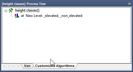
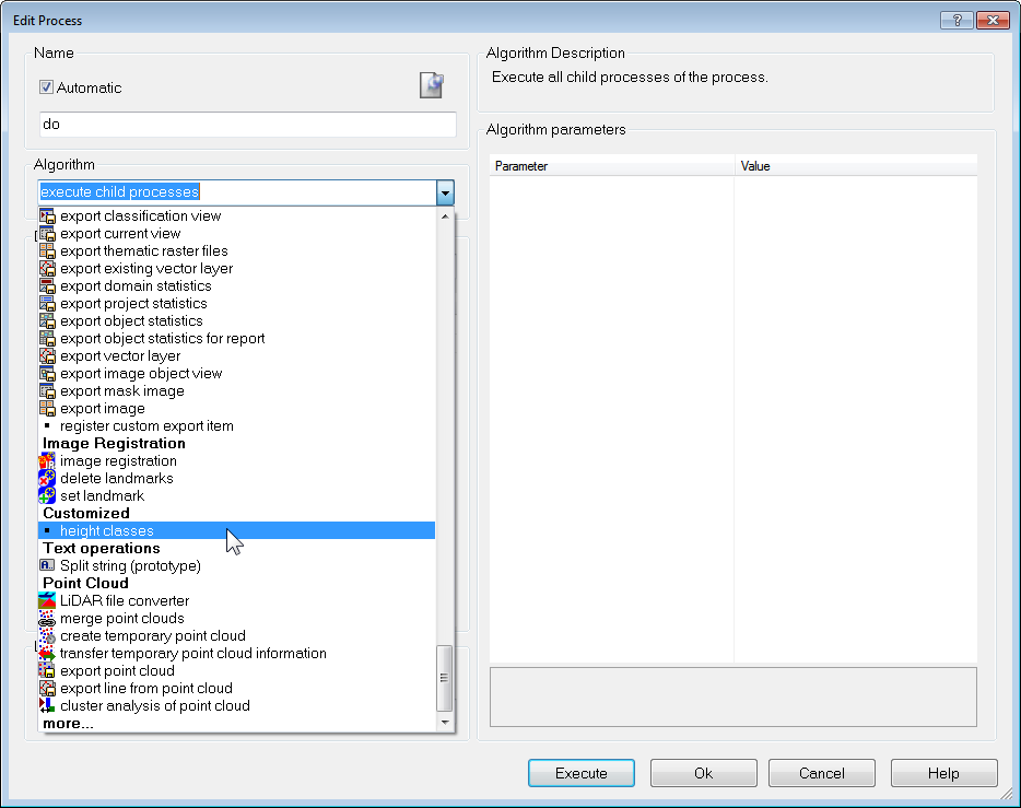
Once you have created a customized algorithm, it displays in the Customized Algorithms tab of the Edit Process Tree window. The rule set items you specified as Parameter are displayed in parentheses following the algorithm’s name.
Customized algorithms are like any other algorithm; you use them in processes added to your rule set in the same way, and you can delete them in the same ways. They are grouped as Customized in the Algorithm drop-down list of the Edit Process dialog box.
You use them in processes added to your rule set in the same way, and you can delete them in the same ways. They are grouped as Customized in the Algorithm drop-down list of the Edit Process dialog box. If a customized algorithm contains parameters, you can set the values in the Edit Process dialog box.
You can edit existing customized algorithms like any other process sequence in the software. That is, you can modify all properties of the customized algorithm using the Customized Algorithm Properties dialog box. To modify a customized algorithm select it on the Customized Algorithms tab of the Process Tree window. Do one of the following to open the Customized Algorithm Properties dialog box:
You can execute a customized algorithm or its child processes like any other process sequence in the software.
Select the customized algorithm or one of its child processes in the Customized Algorithm tab, then select Execute. The selected process tree is executed. The application uses the current settings for all local variables during execution. You can modify the value of all local variables, including parameters, in the Manage Variables dialog box.
If you use the Pass domain from calling process as a parameter domain handling mode, you additionally have to specify the domain that should be used for manual execution. Select the customized algorithm and do one of the following:
To delete a customized algorithm, select it on the Customized Algorithms tab of the Process Tree window. Do one of the following:
The customized algorithm is removed from all processes of the rule set and is also deleted from the list of algorithms in the Edit Process dialog box.
Customized algorithms and all processes that use them are deleted without reconfirmation.
You can save a customized algorithm like any regular process, and then load it into another rule set.
As explained in chapter one, a project can contain multiple maps. A map can:
In contrast to workspace automation, maps cannot be analyzed in parallel; however, they allow you to transfer the image object hierarchy. This makes them valuable in the following use cases:
When working with maps, make sure that you always refer to the correct map in the domain. The first map is always called ‘main’. All child processes using a ‘From Parent’ map will use the map defined in a parent process. If there is none defined then the main map is used. The active map is the map that is currently displayed and activated in Map View – this setting is commonly used in Architect solutions. The domain Maps allows you to loop over all maps fulfilling the set conditions.
Be aware that increasing the number of maps requires more memory and the eCognition client may not be able to process a project if it has too many maps or too many large maps, in combination with a high number of image objects. Using workspace automation splits the memory load by creating multiple projects.
Use cases that require different images to be loaded into one project, so-called multi-project maps, are commonly found:
There are two ways to create a multi-project:
Like workspace automation, a copy of a map can be used for multiscale image analysis – this can be done using the Copy Map algorithm. The most frequently used options are:
When defining the source map to be copied you can:
The third option creates a map that has the extent of a bounding box drawn around the image object. You can create copies of any map, and make copies of copies. eCognition Developer maps can be copied completely or 2D subsets can be created. Copying image layer or image objects to an already existing map overwrites it completely. This also applies to the main map, when it is used as target map. Therefore, image layers and thematic layers can be modified or deleted if the source map contains different image layers.
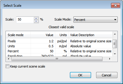
Use the Scale parameter to define the scale of the new map. Keep in mind that there are absolute and relative scale modes. For instance, using magnification creates a map with a set scale, for example 2x, with reference to the original project map. Using the Percent parameter, however, creates a map with a scale relative to the selected source map. When downsampling maps, make sure to stay above the minimum size (which is  ). In case you cannot estimate the size of your image data, use a scale variable with a precalculated value in order to avoid inadequate map sizes.
Resampling is applied to the image data of the target map to be downsampled. The Resampling parameter allows you to choose between the following two methods:
In order to display different maps in the Map View, switch between maps using the Select active map drop-down menu in the navigate toolb ar. To display several maps at once, use the Split commands available in the Window menu.
When working with multi-scale or multi-project maps, you will often want to transfer a segmentation result from one map to another. The Synchronize Map algorithm allows you to transfer an image object hierarchy using the following settings:
Synchronize Map is most useful when transferring image objects of selected image object levels or regions. When synchronizing a level into the position of a super-level, then the relevant sub-objects are modified in order to maintain a correct image object hierarchy. Image layers and thematic layers are not altered when synchronizing maps.
Maps are automatically saved when saving the project. Maps are deleted using the Delete Map algorithm. You can delete each map individually using the domain Execute, or delete all maps with certain prefixes and defined conditions using the domain maps.
Creating a downsampled map copy is useful if working on a large image data set when looking for regions of interest. Reducing the resolution of an image can improve performance when analyzing large projects. This multi-scale workflow may follow the following scheme.
Likewise you can also create a scene subset in a higher scale from the downsampled map. For more information on scene subsets, refer to Workspace Automation.
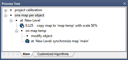
In some use cases it makes sense to refine the segmentation and classification of individual objects. The following example provides a general workflow. It assumes that the objects of interest have been found in a previous step similar to the workflow explained in the previous section. In order to analyze each image object individually on a separate map do the following:
Detailed processing of high-resolution images can be time-consuming and sometimes impractical due to memory limitations. In addition, often only part of an image needs to be analyzed. Therefore, workspace automation enables you to automate user operations such as the manual selection of subsets that represent regions of interest. More importantly, multi-scale workflows – which integrate analysis of images at different magnifications and resolutions – can also be automated.
Within workspace automation, different kinds of scene copies, also referred to as sub-scenes, are available:
Sub-scenes let you work on parts of images or rescaled copies of scenes. Most use cases require nested approaches such as creating tiles of a number of subsets. After processing the sub-scenes, you can stitch the results back into the source scene to obtain a statistical summary of your scene.
In contrast to working with maps, workspace automation allows you to analyze sub-scenes concurrently, as each sub-scene is handled as an individual project in the workspace. Workspace automation can only be carried out in a workspace.
A scene copy is a duplicate of a project with image layers and thematic layers, but without any results such as image objects, classes or variables. (If you want to transfer results to a scene copy, you might want to use maps. Otherwise you must first export a thematic layer describing the results.)
Scene copies are regular scene copies if they have been created at the same magnification or resolution as the original image (top scene). A rescaled scene copy is a copy of a scene at a higher or lower magnification or resolution.
To create a regular or rescaled scene copy, you can:
The scene copy is created as a sub-scene below the project in the workspace.
A scene subset is a project that contains only a subset area (region of interest) of the original scene. It contains all image layers and thematic layers and can be rescaled. Scene subsets used in workspace automation are created using the Create Scene Subset algorithm. Depending on the selected domain of the process, you can define the size and cutout position.
Neighboring image objects of the selected classes, which are located inside the cutout rectangle, are also copied to the scene subset. You can choose to exclude them from further processing by giving the parameter Exclude Other Image Objects a value of Yes. If Exclude Other Image Objects is set to Yes, any segmentation in the scene subset will only happen within the area of the image object used for defining the subset. Results are not transferred to scene subsets.
The scene subset is created as a sub-scene below the project in the workspace. Scene subsets can be created from any data set.
Sometimes, a complete map needs to be analyzed, but its large file size makes a straightforward segmentation very time-consuming or processor-intensive. In this case, creating scene tiles is a useful strategy. Creating scene tiles cuts the selected scene into equally sized pieces. To create a scene tile you can:
Define the tile size for x and y; the minimum size is 100 pixels. Scene tiles cannot be rescaled and are created in the magnification or resolution of the selected scene. Each scene tile will be a sub-scene of the parent project in the workspace. Results are not included in the created tiles.
Scene tiles can be created from any data set. When tiling videos (time series), each frame is tiled individually.
Manually created scene copies are added to the workspace as sub-scenes of the originating project. Image objects or other results are not copied into these scene copies.
Click the Image View or Project Pixel View button on the View Settings toolbar to display the map at the original scene scale. Switch between the display of the map at the original scene scale (button activated) and the rescaled resolution (button released).
Manually created scene tiles are added into the workspace as sub-scenes of the originating project. Image objects or other results are not copied into these scene copies.
You can analyze tile projects in the same way as regular projects by selecting single or multiple tiles or folders that contain tiles.
In the Workspace window, select a project with a scene from which you created tiles or subsets. These tiles must have already been analyzed and be in the ‘processed’ state. To open the Stitch Tile Results dialog box, select Analysis > Stitch Projects from the main menu or right-click in the workspace window.
The Job Scheduler field lets you specify the computer that is performing the analysis. It is set to http://localhost:8184 by default, which is the local machine. However, if you are running an eCognition Server over a network, you may need to change this field.
Click Load to load a ruleware file for image analysis – this can be a process (.dcp) or solution (.dax) file that contains a rule set to apply to the stitched projects.
For more details, see Submitting Batch Jobs to a Server.
The concept of workspace automation is realized by structuring rule sets into subroutines that contain algorithms for analyzing selected sub-scenes.
Workspace automation can only be done on an eCognition Server. Rule sets that include subroutines cannot be run in eCognition Developer in one go. For each subroutine, the according sub-scene must be opened.
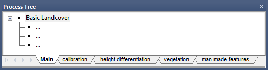
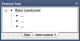
A subroutine is a separate part of the rule set, cut off from the main process tree and applied to sub-scenes such as scene tiles. They are arranged in tabs of the Process Tree window. Subroutines organize processing steps of sub-scenes for automated processing. Structuring a rule set into subroutines allows you to focus or limit analysis tasks to regions of interest.
The general workflow of workspace automation is as follows:
A rule set with subroutines can be executed only on data loaded in a workspace. Processing a rule set containing workspace automation on an eCognition Server allows simultaneous analysis of the sub-scenes submitted to a subroutine. Each sub-scene will then be processed by one of the available engines.
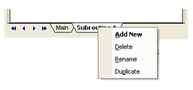
To create a subroutine, right-click on either the main or subroutine tab in the Process Tree window and select Add New. The new tab can be renamed, deleted and duplicated. The procedure for adding processes is identical to using the main tab.
Developing and debugging open projects using a step-by-step execution of single processes is appropriate when working within a subroutine, but does not work across subroutines. To execute a subroutine in eCognition Developer, ensure the correct sub-scene is open, then switch to the subroutine tab and execute the processes.
When running a rule set on an eCognition Server, subroutines are automatically executed when they are called by the Submit Scenes for Analysis algorithm (for a more detailed explanation, consult the eCognition Developer Reference Book).
Right-clicking a subroutine tab of the Process Tree window allows you to select common editing commands.
You can move a process, including all child processes, from one subroutine to another subroutine using copy and paste commands. Subroutines are saved together with the rule set; right-click in the Process Tree window and select Save Rule Set from the context menu.
The strategy behind analyzing large images using workspace automation depends on the properties of your image and the goal of your image analysis. Most likely, you will have one of the following use cases:
To give you practical illustrations of structuring a rule set into subroutines, refer to the use cases in the next section, which include samples of rule set code. For detailed instructions, see the related instructional sections and the algorithm settings in the eCognition Developer Reference Book.
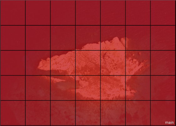
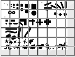
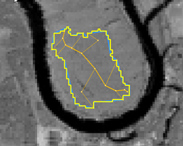
Tiling an image is useful when an analysis of the complete image is problematic. Tiling creates small copies of the image in sub-scenes below the original image. (For an example of a tiled top scene, see the figure below). Each square represents a scene tile.
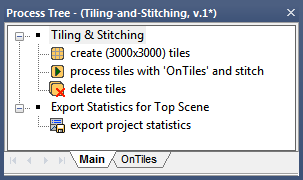
In order to put the individually analyzed tiles back together, stitching is required. Exemplary rule sets can be found in the eCognition User Community (e.g. User Community - Tiling and Stitching). A complete workflow and implementation in the Process Tree window is illustrated here:
Only the main map of tile projects can be stitched together.
In this basic use case, a subroutine limits detailed analysis to subsets representing ROIs – this leads to faster processing.
Commonly, such subroutines are used at the beginning of rule sets and are part of the main process tree on the Main tab. Within the main process tree, you sequence processes in order to find ROIs against a background. Let us say that the intermediate results are multiple image objects of a class ‘no_background’, representing the regions of interest of your image analysis task.
While still editing in the main process tree, you can add a process applying the Create Scene Subset algorithm on image objects of the class ‘no_background’ in order to analyze ROIs only.
The subsets created must be sent to a subroutine for analysis. Add a process with the algorithm Submit Scenes for Analysis to the end of the main process tree; this executes a subroutine that defines the detailed image analysis processing on a separate tab.
Creating scene copies and scene subsets is useful if working on a large image data set with only a small region of interest. Scene copies are used to downscale the image data. Scene subsets are created from the region of interest at a preferred magnification or resolution. Reducing the resolution of an image can improve performance when analyzing large projects.
In eCognition Developer you can start an image analysis on a low-resolution copy of a map to identify structures and regions of interest. All further image analyses can then be done on higher-resolution scenes. For each region of interest, a new subset project of the scene is created at high resolution. The final detailed image analysis takes place on those subset scenes. This multi-scale workflow can follow the following scheme.
| Workflow | Subroutine | Key Algorithm | |
|---|---|---|---|
| 1 | Create a scene copy at lower magnification | Main | Create Scene Copy |
| 2 | Find regions of interest (ROIs) | Create rescaled subsets of ROIs | Common image analysis algorithms |
| 3 | Create subsets of ROIs at higher magnification | Create rescaled subsets of ROIs | Create Scene Subset |
| 4 | Tile subsets | Tiling and stitching of subsets | Create Scene Tiles |
| 5 | Detailed analysis of tiles | Detailed analysis of tiles | Several |
| 6 | Stitch tile results to subset results | Detailed analysis of tiles | Submit Scenes for Analysis |
| 7 | Merge subsets results back to main scene | Create rescaled subsets of ROIs | Submit Scenes for Analysis |
| 8 | Export results of main scene | Export results of main scene | Export Classification View |
This workflow could act as a prototype of an analysis automation of an image at different magnifications or resolutions. However, when developing rule sets with subroutines, you must create a specific sequence tailored to your image analysis problem.
Create a rescaled scene copy at a lower magnification or resolution and submit for processing to find regions of interest.
In this use case, you use a subroutine to rescale the image at a lower magnification or resolution before finding regions of interest (ROIs). In this way, you reduce the amount of image data that needs to be processed and your process consumes less time and performance. For the first process, use the Create Scene Copy algorithm.
With the second process – based on the Submit Scenes for Analysis algorithm – you submit the newly created scene copy to a new subroutine for finding ROIs at a lower scale.
When working with subroutines you can merge back selected results to the main scene. This enables you to reintegrate results into the complete image and export them together. To fulfill a prerequisite to merging results back to the main scene, set the Stitch Subscenes parameter to Yes in the Submit Scenes Analysis algorithm.
In this step, you use a subroutine to find regions of interest (ROIs) and classify them, in this example, as ‘ROI’.
Based on the image objects representing the ROIs, you create scene subsets of the ROIs. Using the Create Scene Subset algorithm, you can rescale them to a higher magnification or resolution. This scale will require more processing performance and time, but it also allows a more detailed analysis.
Finally, submit the newly created rescaled subset copies of regions of interest for further processing to the next subroutine. Use the Submit Scenes for Analysis algorithm for such connections of subroutines.
Create Rescaled Subsets of ROI Find Regions of Interest (ROI) ... ... ... ROI at ROI_Level: create subset 'ROI_Subset' with scale 40x process 'ROI_Subset*' subsets with 'Tiling+Stitching of Subsets' and stitch with 'Export Results of Main Scene'
Create tiles, submit for processing, and stitch the result tiles for post-processing. In this step, you create tiles using the Create Scene Tiles algorithm.
In this example, the Submit Scenes for Analysis algorithm subjects the tiles to time- and performance-consuming processing which, in our example, is a detailed image analysis at a higher scale. Generally, creating tiles before processing enables the distribution of the analysis processing on multiple instances of Analysis Engine software.
Here, following processing of the detailed analysis within a separate subroutine, the tile results are stitched and submitted for post-processing to the next subroutine. Stitching settings are done using the parameters of the Submit Scenes for Analysis algorithm.
Tiling+Stitching Subsets create (500x500) tiles process tiles with 'Detailed Analysis of Tiles' and stitch Detailed Analysis of Tiles Detailed Analysis ... ... ...
If you want to transfer result information from one sub-scene to another, you can do so by exporting the image objects to thematic layers and adding this thematic layer then to the new scene copy. Here, you either use the Export Vector Layer or the Export Thematic Raster Files algorithm to export a geocoded thematic layer. Add features to the thematic layer in order to have them available in the new scene copy.
After exporting a geocoded thematic layer for each subset copy, add the export item names of the exported thematic layers in the Additional Thematic Layers parameter of the Create Scene Tiles algorithm. The thematic layers are matched correctly to the scene tiles because they are geocoded.
Using the submit scenes for analysis algorithm, you finally submit the tiles for further processing to the subsequent subroutine. Here you can utilize the thematic layer information by using thematic attribute features or thematic layer operations algorithms.
Likewise, you can also pass parameter sets to new sub-scenes and use the variables from these parameter sets in your image analysis.
Sub-scenes can be tiles, copies or subsets. You can export statistics from a sub-scene analysis for each scene, and collect and merge the statistical results of multiple files. The advantage is that you do not need to stitch the sub-scenes results for result operations concerning the main scene.
To do this, each sub-scene analysis must have had at least one project or domain statistic exported. All preceding sub-scene analysis, including export, must have been processed completely before the Read Subscene Statistics algorithm starts any result summary calculations. Result calculations can be performed:
After processing all sub-scenes, the algorithm reads the exported result statistics of the sub-scenes and performs a defined mathematical summary operation. The resulting value, representing the statistical results of the main scene, is stored as a variable. This variable can be used for further calculations or export operations concerning the main scene.
Hierarchical image object levels allow you to derive statistical information about groups of image objects that relate to super-, neighbor- or sub-objects. In addition, you can derive statistical information from groups of objects that are linked to each other. Use cases that require you to link objects in different image areas without generating a common super-object include:
The concept of creating and working with image object links is similar to analyzing hierarchical image objects, where an image object has ‘virtual’ links to its sub- or superobjects. Creating these object links allows you to virtually connect objects in different maps and areas of the image. In addition, object links are created with direction information that can distinguish between incoming and outgoing links, which is an important feature for object tracking.
Through the tutorials in earlier chapters, you will already have some familiarity with the idea of parent and child domains, which were used to organize processes in the Process Tree. In that example, a parent object was created which utilized the Execute Child Processes algorithm on the child processes beneath it.
The child processes within these parents typically defined algorithms at the image object level. However, depending on your selection, eCognition Developer can apply algorithms to other objects selected from the Domain.
Object Links are created using the Create links algorithm. Links may link objects on different hierarchical levels, different frames or on different maps. Therefore, an image object can have any number of object links to any other image object. A link belongs to the level of its source image object.
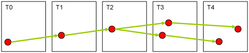
The direction of a link is always directed towards the target object, so is defined as an incoming link. The example in the figure below shows multiple time frames (T0 to T4). The object (red) in T2 has one incoming link and two outgoing links. In most use cases, multiple links are created in a row (defined as a path). If multiple links are connected to one another, the link direction is defined as:
The length of a path is described by a distance. Linked object features use the max. distance parameter as a condition. Using the example in the figure below, distances are counted as follows:
An object link is stored in a class, called the link class. These classes appear as normal classes in the class hierarchy and groups of links can be distinguished by their link classes. When creating links, the domain defines the source object and the candidate object parameters define the target objects. The target area is set with the Overlap Settings parameters.
Existing links are handled in this way:
 new links (which are clones of the old ones)
 When linking objects in different maps, it may be necessary to apply transformation parameters – an example is where two images of the same object are taken by different devices. You can specify a parameter set defining an affine transformation between the source and target domains of the form ax + b, where a is the transformation matrix and b is the translation vector.
By default all object links of an image object are outlined when selecting the image object in the Map View. You can display a specific link class, link direction, or links within a maximal distance using the Edit Linked Object Visualization dialog. Access the dialog in the Menu: View – Display Mode - Edit Linked Object Visualization.
For creating statistics about linked objects, eCognition Developer provides Linked Objects Features:
Polygons are vector objects that provide more detailed information for characterization of image objects based on shape. They are also needed to visualize and export image object outlines. Skeletons, which describe the inner structure of a polygon, help to describe an object’s shape more accurately.
Polygon and skeleton features are used to define class descriptions or refine segmentations. They are particularly suited to studying objects with edges and corners.
A number of shape features based on polygons and skeletons are available. These features are used in the same way as other features. They are available in the feature tree under Object Features > Geometry > Based on Polygons or Object Features > Geometry > Based on Skeletons.
Polygon and skeleton features may be hidden – to display them, go to View > Customize and reset the View toolbar.
Polygons are available after the first segmentation of a map. To display polygons in the map view, click the Show/Hide Polygons button (if activated deactivate Show or Hide outlines button first). For further options, open View > Display Mode > Edit Highlight Colors.
If the polygons cannot be clearly distinguished due to a low zoom value, they are automatically deactivated in the display. In that case, choose a higher zoom value.
Skeletons are automatically generated in conjunction with polygons. To display skeletons, click the Show/Hide Skeletons button and select an object. You can change the skeleton color in the Edit Highlight Colors settings.
To view skeletons of multiple objects, draw a polygon or rectangle, using the Manual Editing toolbar to select the desired objects and activate the skeleton view.
Skeletons describe the inner structure of an object. By creating skeletons, the object’s shape can be described in a different way. To obtain skeletons, a Delaunay triangulation of the objects’ shape polygons is performed. The skeletons are then created by identifying the mid-points of the triangles and connecting them. To find skeleton branches, three types of triangles are created:
The main line of a skeleton is represented by the longest possible connection of branch points. Beginning with the main line, the connected lines then are ordered according to their types of connecting points.
The branch order is comparable to the stream order of a river network. Each branch obtains an appropriate order value; the main line always holds a value of 0 while the outmost branches have the highest values, depending on the objects’ complexity.

The right image shows a skeleton with the following branch order:
Encrypting rule sets prevents others from reading and modifying them. To encrypt a rule set, first load it into the Process Tree window. Open the Process menu in the main menu and select Encrypt Rule Set to open the Encrypt Data dialog box. Enter the password that you will use to decrypt the rule set and confirm it.
The rule set will display only the parent process, with a padlock icon next to it. If you have more than one parent process at the top level, each of them will have a lock next to it. You will not be able to open the rule set to read or modify it, but you can append more processes to it and they can be encrypted separately, if you wish.
Decrypting a rule set is essentially the same process; first load it into the Process Tree window, then open the Process menu in the main menu bar and select Decrypt Rule Set to open the Decrypt Data dialog box. When you enter your password, the padlock icon will disappear and you will be able to read and modify the processes.
If the rule set is part of a project and you close the project without saving changes, the rule set will be decrypted again when you reopen the project. The License id field of the Encrypt Data dialog box is used to restrict use of the rule set to specific eCognition licensees. Simply leave it blank when you encrypt a rule set.
1 As with class-related features, the relations refer to the group hierarchy. This means if a relation refers to one class, it automatically refers to all its subclasses in the group hierarchy. (↑)
2 Customized features that are based on class-related features cannot be saved by using the Save Customized Features menu option. They must be saved with a rule set. (↑)
© 2019, Trimble Inc. All rights reserved. 